Conditional Variational Autoencoders (or CVAEs for short) are a really powerful and creative tool in AI. To really get to the heart of how they work, it's helpful to understand Autoencoder (AE) first. We’ll then move to Variational Autoencoders (VAEs), which are themselves a special version of the basic AutoEncoder.

At its core, an Autoencoder is a type of neural network that learns to do two things:

1. Encode: Compress data into a smaller representation.
2. Decode: Reconstruct the original data from that compressed version.

• The Encoder takes the input (e.g., a high-resolution image) and compresses it down to a low-dimensional "summary." This compressed summary is called the bottleneck or latent space.
• The Decoder takes this compressed summary and tries to reconstruct the original image.

The entire network is trained by comparing the final output to the original input. The goal is to make the reconstruction as close to the original as possible. The bottleneck is intentionally small, the autoencoder is forced to learn the most essential and distinctive features of the data and throw away the non-essential "noise."

An input image of a '7' is made of 784 pixels (a 28x28 grid). The encoder might be forced to compress this down to, say, just 32 numbers. To do this successfully, it can't memorize the pixels. It has to learn the abstract idea of a '7': "a horizontal line at the top connected to a diagonal line going down." The specific thickness of the line or the exact angle are noise it learns to ignore. So, a well-trained AE gives us a powerful feature extractor. The compressed representation in the latent space is a rich, meaningful summary of the input.

While the AE's latent space is great for compressing data it has seen, it's not good for generating new data. The space is often disjointed and uneven. The cluster of points representing '1's might be far away from the cluster for '8's, with empty, meaningless gaps in between. If we were to just pick a random point from one of those empty gaps and feed it to the decoder, it would have no idea what to do. The output would likely be a blurry, unrecognizable blob. Can we organize this latent space so that it's smooth and continuous, allowing us to pick any point and generate a plausible new image? This is exactly the problem that a Variational Autoencoder (VAE) is designed to solve.

Awesome. Let's dive into the clever solution offered by the Variational Autoencoder (VAE).

A VAE introduces a brilliant twist to solve the "empty gaps" problem in the latent space. Instead of the encoder outputting a single, precise point (a vector), it outputs the parameters of a probability distribution. Typically, this is a simple Gaussian (or normal) distribution. So, for any given input image, the encoder outputs two things:

1. A mean vector (μ)
2. A log-variance vector $(log(\sigma^2))$

These two vectors define a "fuzzy" region or a cloud of possible points in the latent space. We then sample a point z (in our latent space) from this distribution and pass it to the decoder.

A VAE is trained to balance two competing objectives:

1. Reconstruction Loss: This is the same as in a standard AE. It pushes the decoder to create an output that's as close to the original input as possible. This ensures the generated images are clear and realistic.
2. KL Divergence Loss: This is the magic ingredient! This loss term acts as a regularizer. It measures how much our learned distribution (defined by μ and σ2) differs from a standard normal distribution (a Gaussian with mean 0 and variance 1). It forces all the learned distributions to stay close to the center of the latent space and overlap with each other. Without this , we would have gaps between the distributions for each digit.

By forcing the distributions to overlap, the VAE fills in the gaps between data clusters. The latent space becomes smooth and continuous. Now, the space between the cluster for '1's and '7's contains points that will decode into plausible digit shapes. This structured space is what gives VAEs their generative power. After training, we can throw away the encoder, pick a random point z from the latent space, and the decoder will generate a digit image that looks like it came from the original dataset.

The ultimate goal of the authors of the VAE paper was to build a powerful generative model. The most principled way to do this involves understanding the relationship between an observed data point (x) and its latent representation (z). This relationship is described by the posterior probability p(z∣x), which tells you, "Given this image, what is the likely latent code that generated it?"

According to Bayes' theorem:

$p(z∣x)=(p(x)p(x∣z))/p(z)$

The big problem here is the denominator, p(x), known as the evidence. To calculate it, you have to compute the integral $p(x)=∫p(x∣z)p(z)dz$ . For any non-trivial model, this integral is intractable—it's impossible to compute because it requires summing over an infinitely complex, high-dimensional space.

The solution was to define a simpler approximation of distributions, let's call it $q_ϕ(z∣x)$ (e.g., a Gaussian), controlled by parameters ϕ. The goal then becomes to tune ϕ to make our simple distribution q as "close" as possible to the true, intractable posterior p(z|x).

The standard way to measure the "closeness" between two distributions is the Kullback-Leibler (KL) Divergence. So, the objective became: Minimize $D_{KL}(q_ϕ(z∣x)∣∣p(z∣x))$. Essentially minimize the distance between our approximation and the original distribution.

By definition →

$D_{KL}(q_ϕ(z∣x)∣∣p(z∣x)) = E_{z-q_{\phi}} [log(q_\phi(z|x)) -log(p(z|x)) ]$

Simplifying using Bayes’ rule (with log)

$log(p(z∣x))=log(p(x∣z))+log(p(z))−log(p(x))$

Replace log(p(z∣x)) in the first equation with the expression from the second step.

$D_{KL}(q_ϕ(z∣x)∣∣p(z∣x))=E_{z∼q_ϕ}[log(q_ϕ(z∣x)) -log(p_θ(x∣z))-log(p(z))+log(p(x))]$

Now, we can group the terms inside the expectation. The term log(p(x)) does not depend on z, so it can be pulled out of the expectation.

$D_{KL}(...)=E_{z∼q_ϕ}[log(q_ϕ(z∣x))−log(p(z))]-E_{z∼q_ϕ}[log(p_θ(x∣z))]+log(p(x))$

The first expectation is just the definition of the KL divergence between $q_ϕ(z∣x)$ and the prior p(z).

$D_{KL}(q_ϕ(z∣x)∣∣p(z∣x))=D_{KL}(q_ϕ(z∣x)∣∣p(z)) - E_{z∼q_ϕ}[log(p_θ(x∣z))]+log(p(x))$

Let us combine the 1st and 2nd term on the right side to a negative & re-arrange to →

$D_{KL}(q_ϕ(z∣x)∣∣p(z∣x))= -L(θ,ϕ;x)+log(p(x))$

Now re-arrange the equation to solve for log(p(x)).

$log(p(x))=L(θ,ϕ;x)+D_{KL}(q_ϕ(z∣x)∣∣p(z∣x))$

We want to maximize the likelihood (the probability of observing our data). Since the 2nd term, KL divergence is always greater than 0, the 1st term is always a lower bound on the log-likelihood. That is why it is called evidence lower bound (ELBO). So, maximizing the likelihood can be simplified to maximizing the ELBO.

From the above derivation ,the ELBO can be written as:

$L(θ,ϕ;x)=E_{z∼q_ϕ}[log(p_θ(x∣z))]−D_{KL}(q_ϕ(z∣x)∣∣p(z))$

This equation represents the VAE's loss function (which we aim to maximize, or equivalently, minimize its negative).

• Reconstruction Term: 1st term in the ELBO This term represents the reconstruction quality. It asks: "If I encode my input x into a distribution $q_ϕ(z∣x)$ and then sample a latent code z from it, how likely is the decoder $p_θ(x∣z)$ to reconstruct the original x?" Maximizing this term forces the VAE to be good at reconstructing its input. In practice, for data like images, this is implemented as a Mean Squared Error or Binary Cross-Entropy loss.
• Regularization Term: KL divergence term This term acts as a regularizer for the latent space. It measures the KL divergence between the distribution returned by the encoder, $q_ϕ(z∣x)$, and our simple prior, $p(z)=N(0,I)$. By maximizing this term (i.e., minimizing the KL divergence), we force the encoder to produce distributions that are close to a standard normal distribution. This is what organizes the latent space, preventing gaps and ensuring it's smooth and continuous for generation.

Essentially, we started with reducing the KL Divergence between our intractable posterior distribution & our approximation. Which on simplification decomposed to give us the log likelihood & some other terms. Solving for the log likelihood gave us the lower bound (ELBO) & another KL divergence term. Now the training of a VAE can be reduced to maximizing the ELBO or conversely minimizing the negative of ELBO.

Before we move on to writing the code, there is another problem that we face\ when it comes to training our VAE. We cannot backpropagate through our sampling stage (between the encoder and decoder). You cannot compute the gradient of a probabilistic sampling. Which means anything before the decoder cannot be trained using traditional means. The authors of the original paper came up with a neat little trick to resolve this issue.

Instead of sampling z directly, we sample a random noise vector ϵ from a standard normal distribution, $ϵ∼N(0,I)$. We then compute z as a deterministic function: $z=μ+σ⊙ϵ$. Here, μ and σ (the mean and standard deviation) are the deterministic outputs of the encoder network. This clever trick separates the random part (ϵ) from the network's parameters, allowing gradients to flow through μ and σ to train the encoder. So $dz/d\mu = 1$ and $dz/d\sigma=\epsilon$.

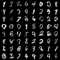
I trained a simple VAE on the MNIST digits dataset. The encoder sends the 28x28 images to a 32 channel convolution layer → ReLU → 64 channel convolution → ReLU → Flatten → 256 channel out Linear layer → ReLU → 20 channel Linear $\mu$ and 20 channel Linear $log(\sigma^2)$. The Decoder is the exact reverse of the encoder, using transposed convolutions in place of convolutions. This complex network trained for 10 epochs ended with a loss of around 65. A sample from this model is below. Not bad, eh!

Let’s move on to Conditional VAEs. The goal of a CVAE is to give us control over the generation process. Instead of asking a VAE to generate a random digit, we want to be able to command it to "generate a 4" or "generate a 9."

The way a CVAE achieves this is surprisingly simple. We feed the "condition"—the piece of information we want to control for (like the digit's label)—as an additional input to both the encoder and the decoder.

This condition is typically represented as a one-hot vector. For example, if we're working with digits 0-9, the label '4' would become the vector [0, 0, 0, 0, 1, 0, 0, 0, 0, 0].

Here’s how it changes the model's job:

• Encoder: Instead of just compressing an image of a '4', the encoder now receives the image and the label '4'. Its job is to encode the unique features of the image that are not explained by the label. In essence, it learns to capture the "style" of the digit (e.g., its slant, thickness, or writer's flair), since it already knows what the digit is.
• Decoder: The decoder receives two inputs: the "style" vector z from the latent space and the condition label '4'. Its job is to use the style information from z to draw the digit specified by the label. It knows what to draw (a '4') and how to draw it (with a specific style).

The ELBO for a CVAE is similar to that of our original VAE →

$L_{CVAE}=E_{z∼q}(z∣x,c)[log(p(x∣z,c))]−D_{KL}(q(z∣x,c)∣∣p(z∣c))$

As you can see, we've simply added the condition ‘c’ to every probability distribution

$p(z|c)$ is the prior that was assumed to be standard normal dist. in our VAE math. For CVAEs, we can still assume a standard normal $N(0,1)$ or we can train another model to give us this prior distribution ⇒ $p(z|c) = N(\mu,\sigma^2)$. We feed in our condition ’c’ and output a $\mu, log(\sigma^2)$. Then we can train all 3 components together; encoder, decoder & the latent prior model.

In most CVAEs, we assume that the "style" (z) should be independent of the "content" or condition (c). For example, the way someone draws a "4" shouldn't fundamentally depend on the fact that it's a "4". Under this assumption, p(z∣c) simplifies to just p(z), which is our good old standard normal distribution, N(0,I).

I trained models with both simple standard normal prior & learned prior. The encoder-decoder is the same architecture as the VAE above with the addition of a one hot encoded class vector representing the digits. The learned prior network is a simple 1 layer ReLU activated feed forward network. I trained both models for 20 epochs.

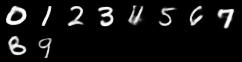
Some samples from the simple CVAE -

Some samples from the Learned Prior CVAE -

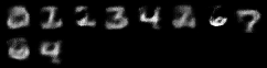
The learned prior CVAE is orders of magnitude worse that the simple CVAE. Sometimes simple is better.

In my next post, we’ll deep dive into some of the popular derivatives of VAEs. Ciao!