This post follows directly from my previous post on Vector Quantised Variational Auto Encoders. The VQ-VAE comprises an encoder that maps observations onto a sequence of discrete latent variables, and a decoder that reconstructs the observations from these discrete variables. Both encoder and decoder use a shared codebook. The encoder produces vectors, the quantiser outputs the nearest vectors for each encoder vector & the decoder uses these quantised vectors to reconstruct the input image. I read about this method from the paper - Neural discrete representation learning by Van den Oord et al.

The original paper talks of VQ VAEs with one quantiser. Encoder → Quantiser → Decoder.

The authors came up with another paper an year later, where they talk of Hierarchical VQ VAEs. In their own words, they propose to use a hierarchy of vector quantized codes to model large images. The main motivation behind this is to model local information, such as texture, separately from global information such as shape and geometry of objects. This lets the different levels separately capture the big picture and the finer details. The top level captures the global features like shape & geometry while the lower level captures local finer details like texture. This "division of labor" seems to be the main motivation behind the Hierarchical VQ VAE. The model learns to encode the big picture and the tiny details separately, and that specialization leads to much higher-quality images.

Encoder (Image to Code)

The encoder's job is to take a high-resolution image and distill it down to a set of codes from our two specialized codebooks (top and bottom). Here’s how it does it, from the bottom up:

1. Input Image: We start with our original image (e.g., a 256x256 picture of a cat).
2. Create Bottom-Level Codes: The encoder first processes the image and shrinks it down, creating a feature map. A smaller feature map that captures a lot of the texture information. It then uses the bottom-level codebook to quantize this map. This gives us the detailed, local description of the image.
3. Create Top-Level Codes: The model takes that first feature map (the one before it was quantized) and processes and shrinks it again. This second, even smaller map now contains only the most essential, high-level structural information. It then uses the top-level codebook to quantize this smaller map. This gives us the abstract, global description.

Decoder (Codes to Image)

Now the decoder gets to work, using both sets of codes to reconstruct the cat picture.

1. Top-Level Codes: The decoder first takes the small, top-level code map (the one defining the img’s overall structure). It upscales this map, turning the global abstraction code into an actual, larger representation of image’s global data. This creates a structural blueprint for the final image.
2. Combine with Bottom-Level Codes: Now, the decoder takes the larger, more detailed bottom-level code map (the "texture" codes). It combines this information with the structural blueprint from the top level. Importantly, the bottom decoder is conditioned on the top-level feature map. The bottom level doesn't have to waste its capacity trying to figure out the global structure all over again. Since the top level has already handled the "big picture," the bottom level can focus all its power on modeling rich, high-fidelity textures.
3. Reconstruct the Image: Using this combined information, the decoder intelligently "paints" the final, high-resolution image. It knows where to put the details because of the top-level structure, and it knows what the details should look like because of the bottom-level texture codes.

Training

The total training objective is a combination of a few key components, applied at each level of the hierarchy (i.e., for both the top and bottom codebooks). It is the same process used by VQ VAEs extended for each level in the Hierarchy.

Reconstruction Loss

This is the most straightforward part. It measures how closely the final output image from the decoder matches the original input image. The model's primary goal is to make this difference as small as possible.

Quantization Loss (Codebook and Commitment)

This is where the magic happens. Since the act of choosing the nearest code from the codebook is like flicking a switch—it's a discrete choice—we can't use standard backpropagation. The model uses two special losses to learn the codebook and guide the encoder:

• Codebook Loss: This loss encourages the chosen vectors in the codebook to move closer to the encoder's output vectors.
• Commitment Loss: This loss does the opposite. It encourages the encoder's output to stay close ("committed") to the codebook vector it chose. This prevents the encoder's outputs from growing arbitrarily large and ensures they are aligned with the learned codebook.

The vector quantization step is non-differentiable. To get the reconstruction error signal back to the encoder, the model uses a straight-through estimator. During the backward pass of training, the gradient skips over the discrete quantization step and is copied directly from the decoder to the encoder.

In the hierarchical model, this entire process is simply done for both the top and bottom levels. The final loss is the reconstruction loss plus the VQ losses for the top codebook and the VQ losses for the bottom codebook, all added together.

Experiments

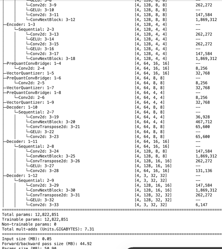
After a couple of weeks of bashing my head against the wall, I was able to create a Hierarchical VQ VAE that was good enough. I used 3 levels instead of 2 and the inverted bottleneck CNN layer from the ConvNext paper. My earlier experiments had all ended in abject failure with reconstructions looking like blurry blobs. The addition of convnext block was the key. The final model had 12 million parameters. I trained it on 2 million 32x32 images of the Cifar100 dataset for 3 epochs. For the first time, I had to shell out to rent a decent GPU for training, all thanks to vast.ai.

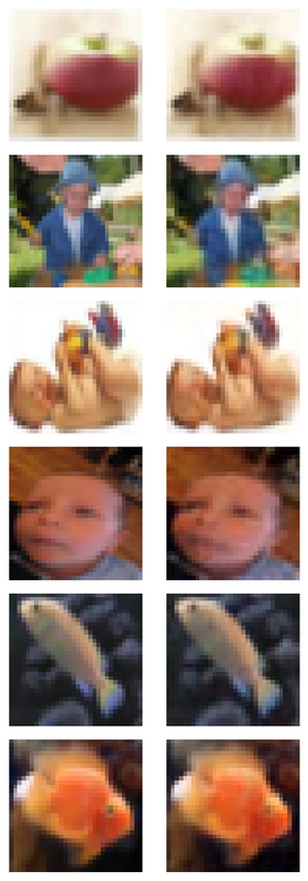
The left column are the original images while the right column are the model reconstructions.

Conditional Priors

After we’ve trained our hierarchical VQ VAE, its encoder can compress any image into a grid of discrete codes (e.g., a 32x32 grid of numbers from 0 to 63). The decoder can turn this grid of codes back into a realistic image. But what if we want to generate a completely new image? We need a way to create a new, valid grid of codes that looks “real”, one that would have come from a real image. We can't just pick random codes, as that would result in nonsense. This is where the prior model comes in. It's a separate model trained on the output of the VQ-VAE encoder. Its only job is to learn the structure and patterns in the compressed code feature maps.

The prior is typically an autoregressive model. This means it generates the grid of codes one by one, where the prediction for the next code depends on all the previous codes it has already generated. A powerful model like a PixelCNN++ or a Transformer is used. These models are excellent at capturing long-range dependencies in data. They use a technique called "masking" to ensure that when predicting a code at a certain position, the model can only see the codes that came before it (e.g., codes above it and to its left). The model is trained to predict the next code in the sequence. For example, given the first 100 codes in a 32x32 grid (1024 total codes), its goal is to predict the 101st code. It learns the conditional probability distribution $P(code_i | code_1,…,code_{i-1})$.

A smaller autoregressive model is trained on the smaller, top-level code maps. This model learns the distribution of the high-level, global structures of the images. A second, much larger autoregressive model is trained on the bottom-level code maps. Crucially, this model is conditioned on the corresponding top-level codes. This means its prediction for a bottom-level detail code depends not only on the previous bottom-level codes but also on the overall structure provided by the entire top-level code map. To generate a new image from scratch, you would first use the top-level prior to generate a complete top-level code map. Then, you would feed that map into the bottom-level prior to generate the detailed bottom-level map. Finally, you would give both of these maps to the HVQ-VAE decoder to generate the final image.

The authors of the original paper used PixelCNN for the priors & so did I. I added a conditioning signal providing the coarse label of the individual images from the Cifar100 dataset. All the priors are CNN models with masked convolutions. The current pixel and every pixel to the right and bottom are zeroed out. This prevents the model from seeing the future pixels. This is a characteristic of autoregressive models. We dont want our model to peek into the future. I also used the Gated Convolution blocks from the authors’ earlier paper. The conditioning signal (class labels) were fed into Residual Conditioning blocks interleaved about the gated convolutions.

All in all, the 3 priors totalled about 1 million parameters. Too small, I know; & the results showed. The conditional generation did not work well. I could not find any papers that condition with 2 signals, the class labels and the other feature maps. I might need more powerful & deeper priors to be able to conditionally generate images. More research needed. The colab notebook for my experiments/training is here.

Sources -

Neural discrete representation learning

Generating Diverse High-Fidelity Images with VQ-VAE-2

ConvNext for the 2020s

Conditional Image Generation with PixelCNN Decoders